Removing the random noise component from the observation, leaving the signal component.
Any number derived from real observation is made up of three components. The first of these is the intended signal, the “perfect” value from the object being observed. The second is error (or noise) caused by environmental disturbance and/or interference. The third is bias, a regular and consistent deviation from the perfect value.
O = S + N + B, or observation equals signal plus noise plus bias
The signal usually is predictably constant, as is the bias. Identifying and eliminating bias requires a set of techniques beyond the scope of this article, so for the remainder of this, we will consider both as components of the signal, leaving a somewhat simpler equation for our observation.
O = S + N, or observation equals signal plus noise
This article focuses on removing the random noise component from the observation and leaving the signal component. The noise is in the form of chance variation, which sometimes enhances the signal and sometimes detracts from it. If we could separate the noise from the signal and eliminate it, our observation would be pure signal, or a precise and consistent value.
Averaging: The simplest routine for removing noise
The first and generally simplest method for obtaining a better observation is averaging. This cannot be used for all conditions, but for many situations it is all that is needed to take very noisy observations and combine them into a remarkably clear and precise measure. It is also a key step in many more complex methods. A critical criterion for this method to be applicable is that the source of the noise is random but stable in nature. If we think of it on a numerical basis, this means that the noise must sometimes increase the number, and sometimes decrease the number, but only within predictable limits.
Let’s look at a simple example where the signal part is the number 4. The noise part is a randomly selected value of –1, 0, or +1. This means that any time this object is observed, we get a number that is either a 3 (4–1), 4 (4–0), or 5 (4+1). This is simulating several observations of the same object. Each reading (O) equals the signal (S) plus the noise (N):
O = S + N
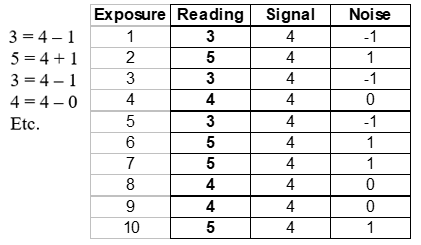
If we add each of these columns, we find that the sum of the readings is 41, the sum of the signal part is 40, but the sum of the noise part is only 1. This is because the negatives and positives in the noise part tend to cancel each other out. If we go back to our original formula, O = S + N, what we have when we sum (Σ) these up is 41 = 40 + 1:
ΣO = Σ(S + N) → ΣO = ΣS + ΣN
To obtain the average, we divide by the number (n) of samples:
ΣO/n = ΣS/n + ΣN/n or
41/10 = 40/10 + 1/10
When we do this, we return to numbers of the original magnitude, but where our noise on individual readings was plus or minus one, our noise on this value is only one-tenth of the original error, or 0.1. (For this particular case, we can expect the residual error to vary as much as ± 0.3, but about 60 percent of the time it will be within ± 0.1 as it was with this sample.) Simply put, the true image stays unchanged, but the noise fades.
The following images graphically demonstrate the power of this simple method. When astronomers do this for each of the pixels in an image, the result is amazingly clear. The following images graphically demonstrate the power of this simple method.
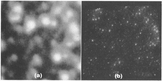
Source: Dinah L. Moche, Astronomy: A Self-Teaching Guide (Wiley, 2014), p. 46
 |
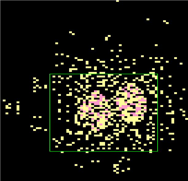
The above illustrations show actual photographs comparing the image obtained with a ground-based telescope to that of the Hubble Space Telescope.
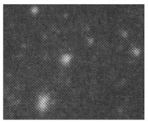
The picture to the right is a blown-up picture from (b) above. In both (a) and the picture to the right, the effects of noise are very apparent. The following illustrations are computer simulations both of noise and correction routines.
The simulation below shows an image that is generated numerically but has a noise component added using a random-number generator. This is essentially an effect that is seen not only on optical images but also on wave sources of any energy level and measurements. The four images that follow show additional random samples from the same source.
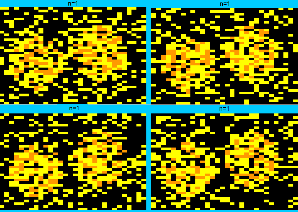
The above images illustrate the random nature of the noise function. A close examination will reveal that each picture is affected differently by noise. Black areas represent background energy levels, yellow represents normal image, and orange represents increased brightness. This variation is a confounding influence that may make a bright spot disappear in one image and may make it appear brighter in another. Although any one of these images is grossly inadequate as a representation, the following pictures—first by averaging four images (n=4), then averaging eight images (n=8)—illustrate the effects of averaging.
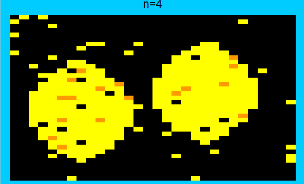
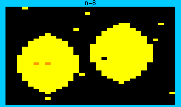
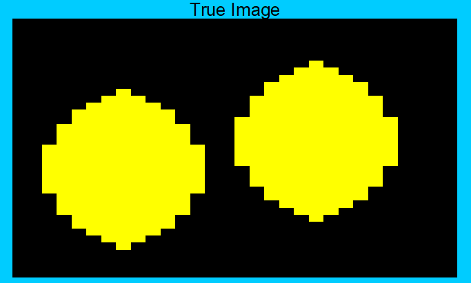
The final image in this series shows the true image that was at the root of the computer simulations. It is quickly apparent that in the “n=8” image, most of the noise has been eliminated leaving a highly purified view of this simulated binary star.
Other implications of this process
As stated earlier, this method is a key step in many other processes. This is because it functions to reduce variation caused by chance. The more random noise that is in an observation, the greater the number of observations that must be averaged to eliminate the noise. However, in any situation where image-to-image (or measurement-to-measurement) variation is high this is the method that will reduce it.
For this particular case, we can expect the residual error to vary as much as ±0.3, but about 60 percent of the time it will be within ±0.1, as it was with this sample.
ABOUT THE AUTHOR

Douglas Allen
Since the early 1980s, Douglas Allen has utilized statistical methods to improve processes and reduce variation. His background includes automotive lighting, electrical connectors and tools for nuclear and aircraft industries, applications in education, and manufacture of personnel care products within the U.S. Food and Drug Administration regulated applications. Allen is currently employed by Edgewell Personal Care.


